Some of the methods described in this chapter take a high dimensional data
matrix as input and give the results as a “rearrangement” of this input. The
rearrangement is usually performed with regard to some similarity or dissimilarity
measure. In clustering algorithms, two relatively similar objects should be
placed in the same cluster. In projection algorithms, they should be placed
in the vicinity of each other in the projected space.
Input to our algorithms is an n x m dimensional matrix with n vectors of length
m. We assume that all vectors are of the same length. When we refer to vector
x in state k, it is generally element (x,k) in the input matrix. We refer to
the distance between vector x and vector y as d(x,y).
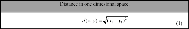
If the input matrix consists of n vectors in 1 state (nx1 dimensional input
matrix) the similarity decision is simple: d(x,y)=|x1-y1|. If vector x has a
value of 3.0 and vector y has a value of 1.0 the distance between them is d(x,y)=3.0
–1.0 = 2.0. The distance from x to y should be the same as the distance from
y to x (symmetric distance), so we define a mathematical equation for the distance
(1):

The most commonly used proximity measure, at least for ratio scales (scales with an absolute 0) is the Minkowski metric (3), which is a generalization of the distance between points in Euclidean space.
The following is a list of the common Minkowski distances for specific values of r:
r = 1. Manhattan /City block distance. A common example of this is the Hamming distance, which is just the number of bits that are different between two binary vectors.
r = 2. Euclidean distance. The most common measure of the distance between two points.
r ![]() "supremum"
(LMAX norm,
L norm)
distance. This is the maximum difference between any component of the vectors.
"supremum"
(LMAX norm,
L norm)
distance. This is the maximum difference between any component of the vectors.
The distance functions implemented in J-Express:
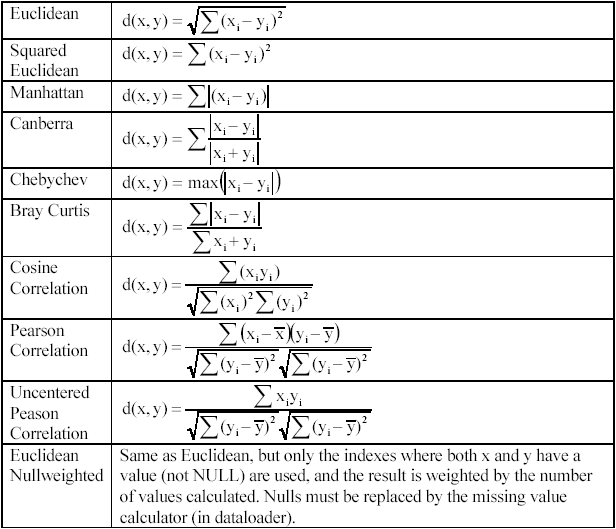
A weakness of the standard Minkowsky distance measure is that if one of the input attributes has a relatively large range, then it can overpower the other attributes. For example, if x0 has a value range of 0-100, and x1 has a value range from 0 to 10, then x0’s influence on the distance function will usually be overpowered by x1’s influence. This is normally not a problem in microarray experiments, as all attributes generally have the same value span. However, to prevent overpowering, the data is often normalized. A simple way of normalizing the vectors is variance and mean normalization, (EQN 7).
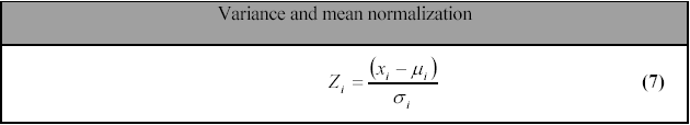
It is very important to understand the effect that normalization has on the data. In the case of equation (7), vectors with very small absolute values will be scaled to have the same variation as vectors with initially very large values (Figure 1). Sometimes this is not desirable.

If we are just looking for profile similarity, that is the shape of the lines, normalization prior to distance calculation is appropriate and allows a simple distance measure (e.g Euclidean) to be used. However, if the absolute value of the vector has some meaning, this will be lost after variance normalization.
Typically, the different distance measures falls into one of two classes: metric and semi-metric. To be classified as ‘metric’, a distance between two vectors x and y must obey several rules:
Distance measures that obey the first three rules, but fail to obey rule 4 are referred to as semi-metric.