Gene Set Enrichment Analysis (GSEA)

Gene Set Enrichment Analysis (Subramanian et al, 2005) is a popular method to use for identifying differentially expressed genes that share some characteristic.

Background

Running GSEA

Interpreting the results

Outputting the results

Background

Gene set analysis is used to look for sets of related genes that follow the same trends in the dataset. It can be performed on either categorical or continuous data. Categorical data is of the type “before” vs “after infection”, while continuous data can be time series data.

Categorical

The traditional way of analysing data for differentially expressed genes has been to use statistics that look at each gene by itself. There are several advantages to analyse sets of genes rather than individual genes.

If the genes only change moderately it may be difficult to find significant change by looking at each gene separately. If, on the other hand, many genes belonging to the same gene set, e.g. immunity and defense, are changed, even moderately, this could be an interesting finding, and the a priori defined relationship between these genes gives more statistical power to detect such smaller changes (affecting a whole set of related genes) compared to a per gene statistic.

It has been common to do simple overrepresentation analysis of for instance GO terms among genes found differentially expressed compared to the non-differentially expressed genes. One would then calculate a per gene statistic, rank the genes and select a cut-off on a certain number of genes or a certain p-value to divide the genes into differentially expressed and non-differentially expressed genes. The per gene individual statistic, and thus the gene expression values themselves, is only used to rank the genes in this approach, not to evaluate the gene sets themselves.

In contrast the gene set enrichment method does not depend on a cut-off, and use the gene expression values of the genes in the evaluation of a gene set. After ranking the genes according to some per gene statistic, the entire ranked list is used to assess how the genes of a gene set distribute across the ranked list. The score (statistic) of individual genes are taken into account when evaluating a set of genes for differential expression.

Imposing a hard cut off on a list of genes with smoothly decreasing statistical scores is bound to be an arbitrary choice, and introduces an artificial border that is oversimplifying the biology. Genes in the area below the cut-off is easily missed that could exhibit the same behavior as related genes in the list above the cut-off.

Continuous

Normally we cluster continuous data to search for genes that have similar expression profiles, and then we go through the genes belonging to a cluster to see if they share some common characteristics. The problem with this approach is that the decision on which cluster a gene is a member of may to some extent be arbitrary, depending on the clustering method, the number of predefined clusters and the intitialisation of the clusters. Some genes that belong to the same geneset may therefor sometimes end up in the same cluster, while other times they end up in different clusters.

Another way continuous data have been analysed has been to search for genes in the dataset with a certain degree of similarity to a particular search profile. Obviously this creates a similar problem as the one described for categorical data; where do we set the cut off? How similar do a profile has to be to make it on to our gene list? All sorts of profiles exist in a data set and it is most likely going to be very difficult to set a clear cut threshold to say that a particular set of genes are similar to the selected profile, while the others are not similar. The resulting limit is therefore always going to be random.

By using a gene search profile and predefined gene sets it is possible to avoid the problems of clustering and setting a cut-off for similarity to a gene profile. We can also get a significance score for each gene set. All the genes in the dataset will then be ranked according to correlation with the search profile. Once the genes have been ranked, the gene sets are scored exactly like they are for categorical data.

Running GSEA

1. Select the dataset in the project tree that you want to run GSEA on
2. Select Gene set enrichment analysis from the Methods | Supervised analysis menu, or click on the (Gene set enrichment analysis) button

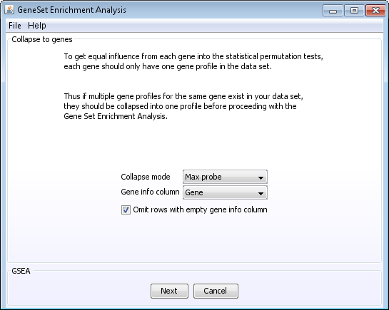
3. Some genes may only have one probe on the array while other genes may have multiple probes on the array. To avoid giving some genesets higher scores based on the number of probes its genes has, it may be a good idea find one profile that can represent the genes with multiple probes. This is called collapsing probes to genes. Creating the new profile can be done in different ways. Choose a collapse mode to select how to create the new gene profile.
   • Collapse modes:
     • Max probe: of all the probes that map to the same gene the value of the probe with the highest intensity is selected
     • Median profile: the median value of all of the probes that map to the same gene is selected.
4. Select the column in your dataset that contains the gene id's.
5. Depending on which gene id you use for Gene info column there may be some blank entries. For instance if you use Gene symbol, not all hypothetical genes that contains probes on your array have gene symbols. These rows can be omitted. The chance that these genes have been mapped to a gene set is lower than for other known transcripts.
6. Click Next NOTE: a new node called Collapsed to genes will now be added to the project tree and the new node is also automatically selected. Important: A bug has been detected related to the automatic selection of the new node, that affects the results if you now continue directly with the next steps. The bug is avoided if you now close the GSEA window, select the collapsed node and open a new GSEA window. Since the new GSEA window will be opened on the already collapsed dataset, you will be taken directly back to the next window.

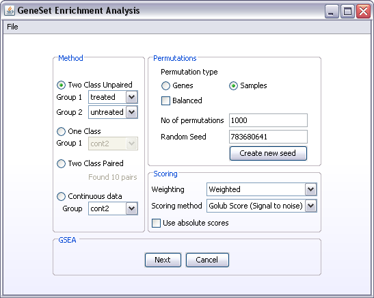
7. Select the appropriate analysis method:
   • Two Class Unpaired: select the two sample groups to be compared from the two drop down lists. If the drop down lists only contain one item (All) you have to define the sample groups from the Create Groups component.
   • One Class: select the sample group to be analysed from the drop down list. If all the samples in your dataset belong to the one sample group you want to analyse, you can select the item All from the dropdown list. If you want to test a sub-group of samples, and the drop down list only contain one item (All), you have to define the sample group from the Create Groups component.
   • Two Class Paired The number of defined pairs in the dataset will be listed under this selection. If no sample pairs are found, you have to define the pairs using the Create groups component.
8. Next select the type of permutation you want to do. If there is enough samples in the dataset, sample permutations will give a more correct estimate of the background distribution of the data. If you have 5 or less samples in each group you are trying to compare a warning will appear saying you should consider gene permutations.
9. Set the number of permutations that should be performed. The number of permutations depend on type of permutation you are doing. Gene permutations will require more permutations than sample permutations. One way of assessing whether you have done enough permutations is to do the analysis again and compare the result. If they are not consistent, more permutations may be needed.
10. Next, select a scoring method. Some of the scoring functions are described here.
11. Weighting means that you value the scores at the top of the ranked list higher than the ones further down the list. An in depth explanantion can be found here.
12. The use of absolute scores means that the up and down regulated genes will be at the top of the list and the non-changing genes will be at the bottom of the list. If you do not use absolute scores the up-regulated genes will be in one end of the list, the down-regulated genes at the other end of the list and the non-changing genes will populate the middle of the list.
13. Click the Next button
14. There are currently two ways of mapping your dataset to different genesets. One is by using the GO tree and the other way is by importing predefined genesets saved in a .gmt file
    • Gene Ontologies can be used as a basis for creating gene sets. To use GO to create gene sets select GO Tree as the Gene Set Source and click on the map dataset to a GO tree button. See here how the GO tree component works.



• Gene sets saved to a .gmt file can also be used. The .gmt file format is explained here. To import a .gmt file select File and click the button to locate the file.



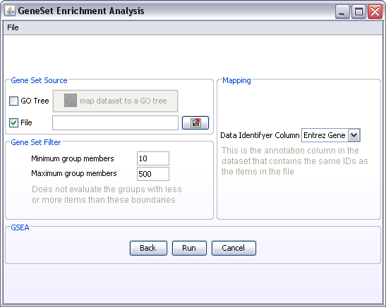
15. Notice that if you select File as your gene set source, the Data Identifyer Column becomes active. To make the connection between the dataset in J-Express and the genes in the gene sets listed in the .gmt file, you must have the same id's that is used in the .gmt file available in the J-Express dataset. Select this column as the Data Identifyer Column. If the correct data column is missing from your J-Express data set, then you can use the Annotation Manager to add it.
16. Gene Set Filter: Very small or very large gene sets should be filtered out. Which limits you use for minimum and maximum depends on how many genes you have in your dataset. For instance: maximum group members of 500 may be ok if you are analysing 20000 genes, but if you are only analysing 2000 genes, then genesets with 500 members may be a bit much.
17. Click Run. Note: before GSEA starts running the genesets will be created and the Gene Set Filters applied to remove small and large genesets. A pop-up window will appear that tells you how many genesets were created, how many were filtered and how many will be used in the analysis. You have to click ok in this window before GSEA starts.

Interpreting the results

An indepth explanation of interpretation of GSEA results can be found on the documentation pages of GSEA at the Broad institute.

Here follows a couple of tips on how to look at the results in J-Express.

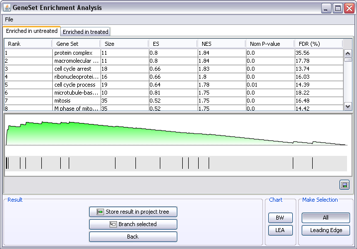
The results are presented in two tabs, one tab for the genesets enriched in each of the groups tested. For paired analysis it will say Enriched in Group 1 and Enriched in Group 2. You can see in the Create Groups window Paired tab which samples belong to Group 1 and Group 2.

1. Each row in the table represents a gene set. Click on a gene set and its "random walk" will be depicted underneath. The peak of the random walk is used as the Enrichment Score (ES) for a gene set.
2. As usual when working in J-Express it is always a good idea to have a Gene Graph open next to the GSEA window. Click on the button to open a Gene Graph or locate it under the Methods | Chart menu.
3. In Gene Graph window: Click the Shadow unselected button.
4. Now when clicking on different gene sets in the GSEA window, the genes belonging to that gene set will be displayed with their gene graphs in the Gene Graph window.
5. The default selection is to view all genes in the dataset that belong to a particular gene set. It is often more useful to only look at the genes that contributed to the Enrichmentscore. This set of genes is called Leading Edge. Click on the Leading Edge button in the GSEA window. Now when selecting different gene sets only the leading edge genes will be displayed in the Gene graph window.

Outputting the results

1. There are different ways of storing the results from the GSEA analysis:
   • Store result in project tree will add a GSEA result node to the project tree, which you can double-click to reopen the result window.
   • Under the file menu of the GSEA window it is possible to save the ordered list of gene sets for the selected tab including the statistical values.
   • Branch off interesting gene sets. To branch off a subdataset containing only the genes in a particular geneset, select the gene set in the GSEA window and click the Branch button.
     • If the All button is selected, the new node in the project tree will contain all genes in the dataset belonging to the particular gene set.
     • If the Leading Edge button is selected, the new node in the project tree will contain only the leading edge genes in the dataset belonging to the particular gene set.
2. Remember to Save the project file from the File menu in the main J-Express window.